Chapter 13 Particle accelerators

13.1 Introduction

In the years immediately following the First World War, there were no particle accelerators. Rutherford’s scattering experiments that led to the discovery of the nucleus, and hence the birth of Nuclear Physics, used $\alpha$ particles produced from radioactive decay. Early accelerators used high voltage generators such as the van de Graaff generator (1931) or the Cockroft and Walton generator (1932) to accelerate particles up to a few MeV. Similar devices are in use to this day as sources of low energy particles. Higher energies require different approaches.

13.2 Basic equations

The relativistic energy of a particle is given by

$$E=m_0\gamma c^2,$$ (13.1)

where $m_0$ is the rest mass, the Lorentz factor is $\gamma ={(1-{\beta }^2)}^{-1/2}$ and $\beta =v/c$. The relativistic momentum of a particle is

$$𝐩=m_0\gamma 𝐯,$$ (13.2)

and the relationship between energy and momentum

$$E^2={𝐩}^2{c}^2+m_0^2{c}^4.$$ (13.3)

where $p=|𝐩|$.

The kinetic energy $T$ is given by

$$T=E-m_0{c}^2=m_0{c}^2(\gamma -1).$$ (13.4)

The Lorentz force of a particle is given by

$$𝐅=\frac{d𝐩}{dt}=q\left(𝐄+𝐯\times 𝐁\right).$$ (13.5)

In an electromagnetic field with $𝐄=0$ and $𝐁⟂𝐯$ the particle will (assuming no energy losses) exhibit circular motion. The magnitude of the relativistic centripetal force is

$$F=\frac{pv}{r},$$ (13.6)

where $r$ is the radius of orbit, so equating with the Lorentz force gives $p=qBr$. For a particle in a uniform, constant magnetic field the radius of orbit is then

$$r=\frac{p}{qB}.$$ (13.7)

A magnetic field does not alter a particles energy. This requires an electric field, and can be easily shown by taking the time derivative of (13.3) and inserting (13.5)

$$E\frac{dE}{dt}=c^2𝐩\cdot \frac{d𝐩}{dt}=q{c}^2𝐩\cdot \left(𝐄+𝐯\times 𝐁\right)=q{c}^2𝐩\cdot 𝐄.$$ (13.8)

The energy gain accelerating through a potential difference of $V$ volts is $qV$.

We will work in units of the electron volt, where $1\mathrm{eV}=1.602\times {10}^{-19}\mathrm{J}$. The rest mass of the electron is 0.511 MeV/$c^2$, the proton 938.3 MeV/$c^2$ and the neutron 939.6 MeV/$c^2$.

13.3 Linear accelerators

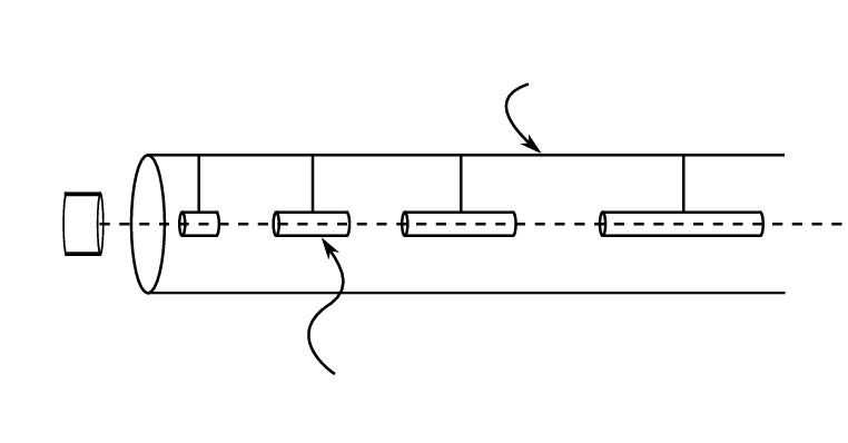
The problem with single stage accelerators is voltage breakdown at the extremely high (few MV) voltages required. This is overcome in the linear accelerator (Wideröe 1927, 1928) by placing a series of cylindrical electrodes (drift tubes) in a straight line. Wideröe realised that if an oscillating voltage is applied to one drift tube flanked by two earthed tubes, and the phase of the voltage changes by ${180}^{\circ }$ during the passage of the particle through the drift tube, it will undergo acceleration at both ends. As the particle accelerates, the drift tubes get progressively longer. This concept was developed by Alvarez in the 1940’s (Fig. 13.1) and accelerators based on this principle are in widespread use today.

Figure 13.1: The Alvarez linac.

The longest linear accelerator is the Stanford Linear Accelerator, some 3 km long, and capable of accelerating electrons to 30 GeV.

The advantages of the LINAC are that no expensive magnetics are needed and there is no energy loss from synchrotron radiation. However, they require many structures and voltage breakdown is still an issue, and accelerating to a large energy requires a long accelerator.

13.4 The cyclotron

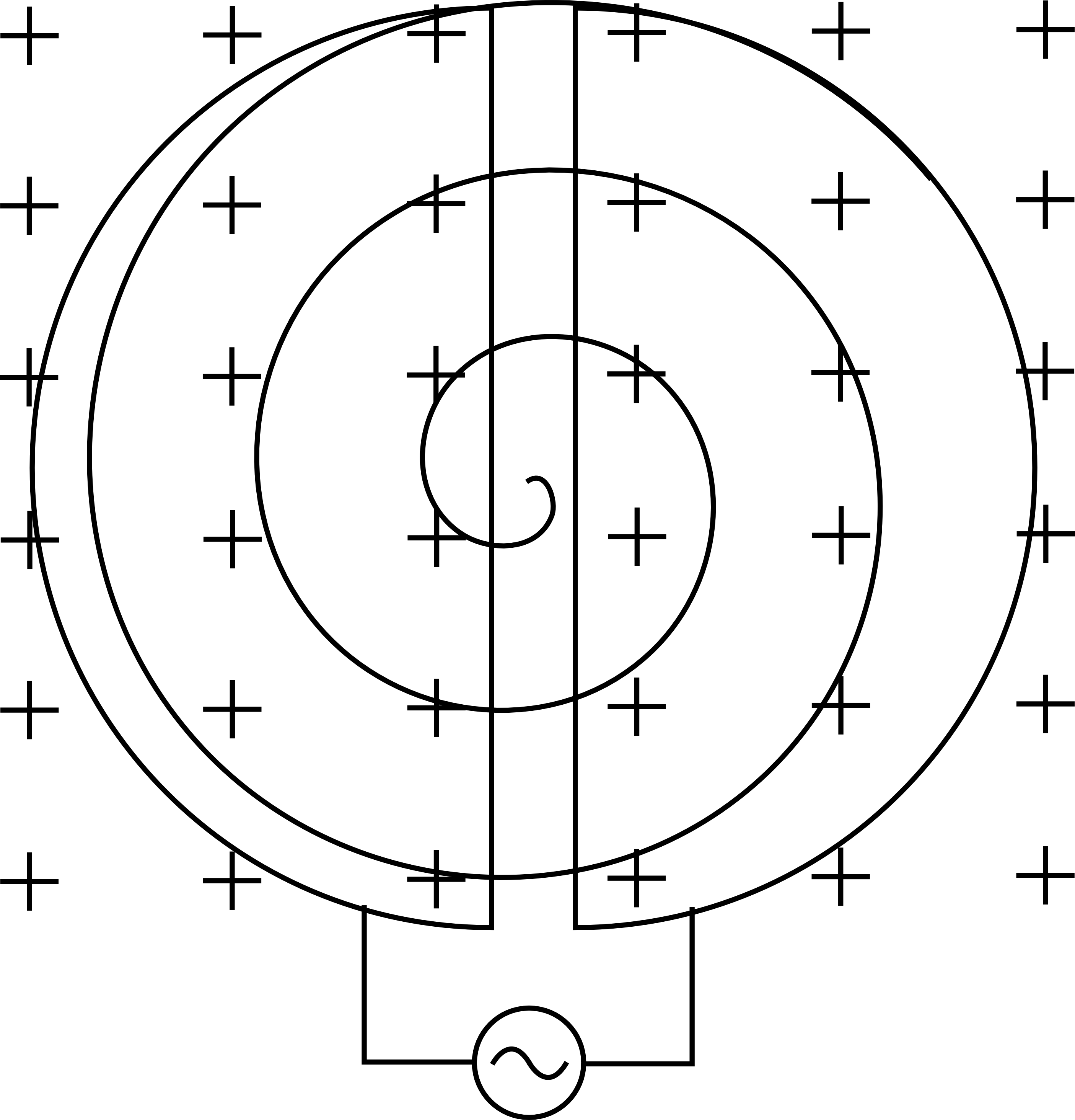
In 1929 Lawrence, working at Berkeley, conceived the cyclotron in which particles are bent into circular paths using a magnetic field. They orbit inside two semi circular chambers or ‘dee’s’ across which an alternating electric field is applied (Fig. 13.2).

Figure 13.2: The principle of the cyclotron. A $B$ field is applied perpendicular to the “dees”.

We can work out the time required for a particle to complete an orbit, and hence the frequency at which the ac voltage should be applied. Using (13.7)

$T={\displaystyle \frac{2\pi r}{v}}={\displaystyle \frac{2\pi p}{vqB}}={\displaystyle \frac{2\pi m}{qB}},$ (13.9)

$f={\displaystyle \frac{1}{T}}={\displaystyle \frac{qB}{2\pi m}},$ (13.10)

where $m=m_0\gamma$ and $f$ is the cyclotron frequency. Notice that this is independent of the radius: as the particle is accelerated and gains energy it spirals out to larger radii. The gain in orbit length is exactly compensated by the gain in velocity. This is the essential feature of the cyclotron. However, as the particles accelerate they eventually reach a velocity where relativistic effects can no longer be ignored. To maintain the cyclotron resonance condition, $B$ must be increased.

If the maximum radius of the cyclotron is R, the maximum velocity and KE of the particle at non-relativistic speeds are

$v_{\max }={\displaystyle \frac{qBR}{m}},$ (13.11)

${\mathrm{KE}}_{\max }={\displaystyle \frac{q^2{B}^2{R}^2}{2m}}$ (13.12)

To achieve high energies large radii and magnetic fields are required. The first cyclotron, built by Lawrence had a radius of 12.5 cm and accelerated protons to an energy of 1.2 MeV. By the late 1930’s radii of 75 cm had been achieved and the energy range extended to $\sim$ 40 MeV.

13.5 The synchrotron

Increasing the energies that can be achieved by conventional cyclotrons is prohibitively expensive as it requires machines with ever larger radii.

However, if the magnetic field and the resonant frequency are both varied, it is possible to arrange for the accelerated particles to orbit at nearly constant radius, requiring a ring shaped magnet. This is the principle of the synchrotron. At relativistic speeds the basic cyclotron condition of (13.10) is modified.

$E=\sqrt{p^2{c}^2+m_0{c}^4},$ (13.13)

$p=qBr,$

$E=\sqrt{q^2{r}^2{B}^2{c}^2+m_0^2{c}^4},$

$f={\displaystyle \frac{qB{c}^2}{2\pi \sqrt{q^2{r}^2{B}^2{c}^2+m_0^2{c}^4}}}.$

This defines the relationship between $B$ and $f$ required to maintain synchronization.

The first proton synchrotron was completed at Brookhaven National Laboratory in 1952. Known as the ‘cosmotron’ it accelerated protons to an energy of 3 GeV. A rival machine, the ‘bevatron’ was constructed at Berkeley. It was designed to accelerate protons to an energy of 6.4 GeV, more than required to produce a proton anti-proton pair. This led to the discovery of the anti-proton in 1956 and to the 1959 Nobel Prize in physics for Chamberlain and Segre.

13.6 Fixed Target and Colliders

Up until the mid 1960’s the accelerated particles were fired at stationary targets. However, this wastes much of the energy in the kinetic energy of the products (required from conservation of momentum considerations). If the particle beams can be made to collide head-on, then all of their energy is available.

13.7 Higher energies

Figure 13.3: Development of high energy accelerators.

Most accelerators are now colliding beam accelerators. However, there is a problem with this approach. The density of particles in a beam bunch is low, typically $\sim {10}^{11}$ particles/cm² and this is to be compared with the density in a stationary target ($\sim {10}^{25}$ particles/cm² for a liquid hydrogen target). Thus reaction rates would be negligibly small. This is solved by storing many accelerator pulses in a storage ring for times $\sim$ 1 day.

In the CERN Intersecting Storage Rings (ISR) beams of 28 GeV protons are directed into two storage rings where they orbit in opposite directions and are made to collide at 8 locations around the ring.

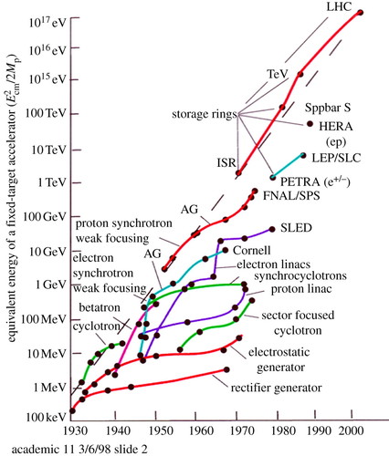
Figure 13.3 charts the development of high energy accelerators. Currently the most powerful collider is CERN’s Large Hadron Collider (LHC). In October 2010 it achieved the target particle density for protons and in 2012 discovered the Higgs boson. It is currently operating with beam energies of 7 TeV, so the available centre of mass energy is 14 TeV using $E_{\mathrm{CM}}=2E_L$. It is now hoping to find evidence of theories such as supersymmetry.